Share valuation is the process of assigning a rupee value to a specific share. An ideal share valuation technique would assign an accurate value to all shares. Share valuation is a complex topic and no single valuation model can truly predict the intrinsic value of a share.
Likewise, no valuation model can predict with certainty how the price of a share will vary in the future. However, valuation models can provide a basis to compare the relative merits of two different shares.
Table of Contents
Common ways for equity valuations could be classified into the following categories:
Earnings Valuation
Earnings (net income or net profit) is the money left after a company meets all its expenditures. To allow for comparisons across companies and time, the measure of earnings is stated as earnings per share (EPS). This figure is arrived at by dividing the earnings by the total number of shares outstanding.
Thus, if a company has one crore shares outstanding and has earned Rs. 2 crore in the past 12 months, it has an EPS of Rs. 2.00.
Rs. 20,000,000/10,000,000 shares = Rs. 2.00 earnings per share
EPS alone would not be able to measure if a company’s share in the market is undervalued or overvalued.
Price/Earnings (P/E) Ratio
Another measure used to arrive at investment valuation is the Price/Earnings (P/E) ratio that relates the market price of a share with its earnings per share. The P/E ratio divides the share price by the EPS of the last four quarters.
For example, if a company is currently trading at Rs. 150 per share with a EPS of Rs. 5 per share, it would have a P/E of 30.
The P/E ratio or multiplier has been used most often to make an investment decision. A high P/E multiplier implies that the market has overvalued the security and a low P/E multiplier gives the impression that the market has undervalued the security. When the P/E multiple is low, it implies that the earnings per share is comparatively higher than the prevailing market price. Hence, the conclusion that the company has been ‘undervalued’ by the market.
Assume a P/E multiplier of 1.0. The implication is that the earnings per share is equal to the prevalent market price. While market price is an expectation of the future worth of the firm, the earnings per share is the current results of the firm. Hence, the notion that the firm has been ‘undervalued’ by the market. On the other hand, a high P/E ratio would imply that the market is ‘overvaluing’ the security for a given level of earnings.
The interpretation of ‘overvaluation’ will hold good when the market is expected to adjust towards the real worth of the company. A consistent high ratio, on the other hand, implies that the future returns expectations from the company is consistently good and that the high P/E ratio need not necessarily indicate a ‘overvalued’ position for the company.
Forward P/E Valuation
The forward P/E valuation is another technique that is based on the assumption that prices adjust to future P/E multipliers. The assumption is that shares typically trade at a constant P/E and therefore the ‘future’ value of a share can be calculated by comparing the current P/E with the future P/E (as predicated using analysts’ estimated earnings for that year).
The forecasted market price is calculated as [Price* (P/E, current)/ (P/E, future)].
For example, if current market price is Rs. 20, the current P/E is 4 and forecasted P/E is 2.5, the forecast price is Rs. 32. [ (20 x 4) / 2.5 ] This valuation technique cannot be applied to shares with negative current or future earnings.
P/E Growth Ratio (PEG)
The forward P/E ratio is most often used in comparison with the current rate of growth in earnings per share. This is based on the assumption that for a growth company, in a fairly valued situation, the price/earnings ratio ought to be equal to the rate of EPS growth. When the growth rate is not in tune with P/E multiplier, then P/E multiplier can be modified to include the growth ratio.
Assume, for example, that a company’s P/E ratio is 15; an earnings growth rate of 13 percent -14 percent would substantiate the fair valuation of the share in the market price. This can be incorporated in the P/E growth ratio (PEG). The PEG considers the annualized rate of growth and compares this with the current share price. Since it is future growth that makes a company valuable to the investors in the market, the earnings growth is expected to depict the valuation of a company better than the historical earnings per share.
If a company is expected to grow at 10 percent a year over the next two years and has a current P/E multiple of 15, the PEG will be computed as 15/10 = 1.5. The interpretation of PEG is that the market price is worth 0.5 times more than what it really is worth, since the assumption is that the P/E multiplier ought to be equal to the earnings growth rate.
A PEG of 1.0 suggests that a company is fairly valued. That is, in the previous example, if the P/E multiplier is 15 and the earnings growth rate is also 15, then PEG is equal to (15/15) 1.0. Here the company is evaluated as priced correctly by the market.
If the company in the above example had a P/E of 15 but was expected to grow at 20 percent a year, it would have a PEG of (15/20), 0.75. This means the shares are selling for 75 percent of their real value. This leads to the conclusion that the shares are ‘underpriced’ in the market.
The PEG measure is useful only for positive growth companies. When the companies are not experiencing a growth opportunity or there is a short spell of negative performance due to various factors, the PEG will not be the right measure to use to assess the valuation of shares.
The forward P/E and growth ratio (FPEG) can be used for valuing companies with expected long-term performance. Rather than looking at the current historical price earning multiplier, the measure considers the price-earnings multiplier forecast by analysts. This is compared with the expected earnings growth rate to evaluate the fair price of the shares.
Assuming the analysts’ expectation of the P/E multiplier of a company is 20 and the earnings growth is expected to be 25 per cent over the next five years, the FPEG is computed as (20/ 25) = 0.8. The interpretation of this number is similar to the interpretation of PEG, that is, the company is evaluated in the market at only 80 per cent of its realistic price. This will be an indicator of ‘underpricing’ of shares in the market.
Similarly, a company that has an expected P/E multiplier of 20 and the growth in earnings in the next five years of 10 per cent will have an FPEG of (20/10) 2.0. This indicates an ‘overpricing’ of the share by the market by double its fair value.
Although the PEG and FPEG are helpful, they both operate on the assumption that the P/E should equal the EPS rate of growth. In the real market, the assumptions behind the earnings valuation methods need not necessarily hold good. A modification to the P/E multiplier approach is to determine the relationship between the company’s P/ E and the average P/E of the stock index. This is called as the price-earnings relative. Price-earnings relative is given by the following formula:
P/E relative = (share P/E)/(Index P/E)
This formula estimates the shares’ P/E movement along with the index P/E. A P/E relative of 1.5 implies that the share is sold in the market 1.5 times that of the index price/earnings.
However, these earnings multipliers become inapplicable when the earnings are negative. Negative earnings cannot be used for valuation of shares. However, when negative earnings occur, appropriate alternative estimates may be used for valuation. The substitute measures would depend on the cause for negative earnings.
There are a number of reasons for a company to have negative earnings. Some of the reasons for negative earnings can be listed as follows:
- Cyclical nature of industry
- Unforeseeable circumstances
- Poor management
- Persistent negative earnings
- High leverage cost
Earnings Forecast
Earnings can be forecast through the forecasts of the rates resulting in the earnings. The variables that can be considered for forecasting earnings can be the future return on assets, expected financial cost (interest cost), the forecasted leverage position (debt-equity ratio), and the future tax obligation of the company. The formula for forecasting the earnings could be stated as follows:
Forecasted earnings (value) = (1-t)*[ROA + (ROA-I)*(D/E)]*E
Where,
ROA = Forecasted return on assets
I = Future interest rate
D = Total expected long term debt
E = Expected equity capital
t = Expected tax rate
Alternatively, a forecast of sales and projected profit margin can be made to compute the forecasted earnings. The sales forecast would depend on the market share of the estimated industry sales forecast. The profit margin forecast will depend on the operational and financial expenses of the company. From this information earnings can be forecast using the following formula:
Forecasted sales = Industry sales target * company’s expected share in industry sales
Forecasted earnings = Forecasted sales * projected profit margin
The third method of forecasting earnings is to identify the individual variables constituting the earnings determination and forecast each of these variables separately. This will involve the forecast of the fixed and variable components of the operational expenses and the financial expense. This method is most applicable when the fixed and variable components of the cost structure of a company do not vary drastically with that of the average industry cost figures.
Consider a company with a high fixed cost relative to that of the industry average. The company will be able to make a positive return only when the projected sales dramatically exceeds this high cost.
The company’s total cost far exceeds the industry total cost. Given a sales level and variable cost level, a company whose fixed costs are above the industry average will be able to reach a profit figure at a comparatively higher level of activity. Similarly, any company that is able to minimise its fixed costs will have a better position in terms of profitability than the industry average. Hence the need to forecast the individual variables that constitute profit rather than the overall return on assets.
Cash Flows Valuation
Cash flows indicate the net of inflows less outflows from operations. Cash flows differ from book profits reported by companies since accounting profits identify expenses that are non-cash items such as depreciation. Cash flows can also be used in the valuation of shares. It is used for valuing public and private companies by investment bankers.
EBDIT
Cash flow is normally defined as earnings before depreciation, interest, taxes, and other amortisation expenses (EBDIT). There are also valuation methods that use free cash flows. Free cash flows is the money earned from operations that a business can use without any constraints. Free cash flows are computed as cash from operations less capital expenditures, which are invested in property, plant and machinery and so on.
EBDIT is relevant since interest income and expense, as well as taxes, are all ignored because cash flow is designed to focus on the operating business and not secondary costs or profits. Taxes especially depend on the legal rules and regulation of a given year and hence can cause dramatic fluctuations in earning power. The company makes tax provisions in the year in which the profits accrue while the real tax payments will be made the following year. This is likely to overstate/ understate the profit of the current year.
Depreciation and amortisation, are called non-cash charges, as the company is not actually spending any money on them. Rather, depreciation is an accounting allocation for tax purposes that allows companies to save on capital expenditures as plant and equipment age by the year or their use deteriorates in value as time goes by.
Amortisation is writing off a capital expenses from current year profit. Such amortised expenses are also the setting aside of profit rather than involving real cash outflows. Considering that they are not actual cash expenditures, rather than accounting profits, cash profits will indicate the real strength of the company while evaluating its worth in the market.
Cash flow is most commonly used to value industries that involve tremendous initial project (capital) expenditures and hence have large amortisation burdens. These companies take a longer time to recoup their initial investments and hence tend to report negative earnings for years due to the huge capital expense, even though their cash flow has actually grown in these years.
The most common valuation application of EBDIT is the discounted cash flow method, where the forecast of cash flows over a period of time are made and these are discounted for their present worth.
The formula for computing the value of the firm will be;
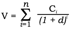
Where,
Ci = cash flows forecast for year i
d = expected rate of return
n = number of years for which forecasts have been made.
This can be easily computed using software applications such as spreadsheet. The following table illustrates the computation of the value of a firm based on cash flow expectations.
| Year | Expected cash flows (Rs. In crore) | Discounted cash flows (Discount rate 12%) (Formula) | Discounted cash flows (Discount Rate 12%) |
|---|---|---|---|
| 1 | 200 | = B2/(1.12)^A2 | 178.57143 |
| 2 | 254 | = B2/(1.12)^A3 | 202.48724 |
| 3 | 236 | = B2/(1.12)^A4 | 167.98014 |
| 4 | 280 | = B2/(1.12)^A5 | 177.94506 |
| 5 | 310 | = B2/(1.12)^A6 | 175.90233 |
| 6 | 324 | = B2/(1.12)^A7 | 164.14848 |
| 7 | 356 | = B2/(1.12)^A8 | 161.03632 |
| 8 | 368 | = B2/(1.12)^A9 | 148.62903 |
| 9 | 375 | = B2/(1.12)^A10 | 135.22876 |
| 10 | 420 | = B2/(1.12)^A11 | 135.22876 |
| 11 | 451 | = B2/(1.12)^A12 | 129.65172 |
| 12 | 473 | = B2/(1.12)^A13 | 121.40732 |
| 13 | 492 | = B2/(1.12)^A14 | 112.7537 |
| 14 | 520 | = B2/(1.12)^A15 | 106.4023 |
| 15 | 534 | = B2/(1.12)^A16 | 97.5598 |
| 16 | 567 | = B2/(1.12)^A17 | 92.4899 |
| 17 | 591 | = B2/(1.12)^A18 | 86.0758 |
| 18 | 612 | = B2/(1.12)^A19 | 79.5842 |
| 19 | 634 | = B2/(1.12)^A20 | 73.6116 |
| 20 | 657 | = B2/(1.12)^A21 | 68.1090 |
| Cash flows No. of shares (in crore) Value per share | = SUM (C2:C21) 200 = (C23/C24) | 2614.8032 200 13.0740 |
Buying a company with good cash flows can yield a lot of benefits to an investor. Cash can fund product development and strategic acquisitions and can be used to meet operational and financial expenditures.
Cash forecasts are made for a limited time duration. However, the shares are valued for their ability to produce an indefinite stream of cash flows. This is referred to as the terminal value of shares. Terminal value usually refers to the value of the company (or equity) at the end of a high growth period. When an indefinite duration of growth is considered, it is normal to assume that a stable growth will follow the high growth. This stable growth rate is expected to remain constant.
With this assumption, the terminal value computation can be given by the following formula:
Terminal value in year n = Cash flow in year (n + 1)/(d – g)
Where,
‘d’ is the discount rate of the cash flows
‘g’ is the stable growth rate
This approach also requires the assumption that growth is constant forever, and that the cost of capital (discount rate) will not change over time.
A stable growth rate is one that can be sustained forever. Since no company, in the long term, can grow faster than the economy that it operates in, a stable growth rate cannot be greater than the growth rate of the economy.
This stable growth rate cannot be greater than the discount rate either because of the risk-free rate that is implied in the discount rate. This invariably means that the discount rate has to be fixed after considering the inflation rate, economic growth rate, time value, and so on.
Price to cash flow ratio can also be used as a valuation model. Cash flow multiplier is computed as: market price/cash flow per share. For example, if the current market price is Rs. 60 and cash flow per share is Rs. 20, the cash flow multiplier would be 3. If the forecasted cash flow per share is Rs. 23, then the market value can be estimated as (23 × 3) Rs. 69.
Economic value added (EVA) is another modification of cash flow that considers the cost of capital and the incremental return above that cost.
Assuming the after tax return from operations is 18% and the cost of capital is 10%, the incremental return for the company would be 8% (18 – 10). If the face value of the investment in the company is Rs. 100 per share, the economic value added per share will be Rs. 8. If the current market price of the share is Rs. 200, then the EVA multiplier will be (200/8) 25. EVA multiple can then be used to identify the under pricing or over pricing of a share in the market.
Asset Valuation
The expectation of earnings and cash flows alone may not be able to identify the correct value of a company. This is because the intangibles such as brand names give credentials for a business. In view of this, investors have begun to consider the valuation of equity through the company’s assets.
Asset valuation is an accounting convention that includes a company’s liquid assets such as cash, immovable assets such as real estate, as well as intangible assets. This is an overall measure of how much liquidation value a company has if all of its assets were sold off. All types of assets, irrespective of whether those assets are office buildings, desks, inventory in the form of products for sale or raw materials and so on are considered for valuation.
Asset valuation gives the exact book value of the company. Book value is the value of a company that can be found on the balance sheet. A company’s total asset value is divided by the current number of shares outstanding to calculate the book value per share. This can also be found through the following method- the value of the total assets of a company less the long-term debt obligations divided by the current number of share outstanding.
The formulas for computing the book value of the share are given below:
Book value = Equity worth (capital including reserves belonging to shareholders)/Number of outstanding shares
Book value = (Total assets – Long-term debt)/Number of outstanding shares
Book value is a simple valuation model. If the investor can buy the shares from the market at a value closer to the book value, it is most valuable to the investor since it is like gaining the assets of the company at cost. However, the extent of revaluation reserve that has been created in the books of the company may distract the true value of assets. The revaluation reserve need not necessarily reflect the true book value of the company; on the other hand, it might be depicting the market price of the assets better.
Book value, however, may not correctly depict the company value, since most companies use different accounting methods. Further, the adjustment to the historical figures in terms of economic inflation or deflation of the asset book values are not incorporated in these value estimations. The book values are also subject to adjustments depending on the tax framework within which the company falls and the consequences relating to the company’s tax planning measures. But, with increased corporate governance practices, the book value concept is becoming more relevant to the investor for valuation purposes.
Another useful measure of asset valuation is the price to book ratio. This ratio is arrived at by relating the current market price of the share to the book value per share. The intention is to compare the prevailing market price with the book value per share and identify if the shares are undervalued or overvalued in the market. The computation of price to book ratio is computed as follows:
Price to book value ratio = Market price/Book value per share.
The undervaluation of shares will be established when the price to book ratio is relatively low. A high price to book ratio, on the other hand, implies that the shares are sold at a price not supported by its asset value in the market.
For example, if a company has total assets less long-term liabilities as Rs. 43950 crores and the number of outstanding shares at 2,000 crores, the book value per share will be (43950/2000) Rs. 21.975. If the market price is quoted at Rs. 84, the Price to Book multiplier will be (84/21.975) 3.82.
Return on Equity (ROE)
Another use of asset valuation is through the return on equity, (ROE). Return on equity is a measure of how much earnings a company generates in four quarters compared to its shareholder’s equity.
For instance, if a company earned Rs. 2 crores in the preceding year and has a shareholder’s equity of Rs. 10 crores, then the ROE is 20 per cent. Investors might use ROE as a filter to select companies that can generate large profits with a relatively small amount as capital investment. The nature of ROE, however, depends on the type of industry the company belongs to. The ROE figures of trading companies are expected to be comparatively higher than that of heavy manufacturing concerns since trading companies need not necessarily require constant capital expenditure.
The book value computation that includes within its fold the valuation of intangible assets such as brands and patents, are viewed positively by investors. Investors view brands as valuable and they are assumed to increase the expected future profits of the company.
Brands also tend to have a strong market potential since customers prefer a brand exclusively for its name and sometimes, brands convey more meaning than the product quality. Specific value is given to brands that have recently established unshakable credentials. Companies also spend a lot of money on building brands in their product portfolios.
Some companies build the brand name around their company name; this has a direct impact on the valuation by companies build the brand name around their company name; this has a direct impact on the valuation by investors. Companies such as Colgate, Intel, Nestle, and Bata have built their company names into brands that give them an incredible edge over their competitors in the market.
Intangibles can also sometimes mean that a company’s shares can trade at a premium to its historical growth rate. Thus, a company with large profit margins, a dominant market share, consistent performance can trade at a slightly higher multiple than its growth rate would otherwise suggest.
A company can sometimes be worth more in reality than when viewed individually in terms of all the assets in its Balance Sheet. Many times, human resource strength is an intangible that is built inside the organisation and neither the company nor the shareholders give a uniform quantification to such strengths. The book valuation process of a company is hence the exercise of a few investment bankers and consultants who get to know the intricate details of the company.
Rather than attempting to make a book valuation of the company individually, investors can rely on such sources to assess the undervaluation or overvaluation of shares in the market.
Dividend Discount Model
According to the dividend discount model, conceptually a very sound approach, the value of an equity share is equal to the present value of dividends expected from its ownership plus the present value of the sale price expected when the equity share is sold. For applying the dividend discount model, we will make the following assumptions:
- dividends are paid annually- this seems to be a common practice for business firms in India; and
- the first dividend is received one year after the equity share is bought.
Single-period valuation model
Let us begin with the case where the investor expects to hold the equity share for one year. The price of the equity share will be:
P0 = [ D1 / (1+r) ] + [ P1 / (1+r) ]
Where, P0= current price of the equity share; D1 = dividend expected a year hence; P1 = price of the share expected a year hence; and r = rate of return required on the equity share.
Expected rate of return
In the preceding discussion we calculated the intrinsic value of an equity share, given information about
- the forecast values of dividend and share price, and
- the required rate of return.
Now we look at a different question: What rate of return can the investor expect, given the current market price and forecast values of dividend and share price? The expected rate of return is equal to:
R = D1/ PO +g
Multi-period valuation Model
Having learnt the basics of equity share valuation in a single-period framework, we now discuss the more realistic, and also the more complex, case of multiperiod valuation.
Since equity shares have no maturity period, they may be expected to bring a dividend stream of infinite duration. Hence the value of an equity share may be put as:
Now, what is the value of Pn in Eq.? Applying the dividend capitalisation principle, the value of Pn, would be the present value of the dividend stream beyond the nth period, evaluated as at the end of the nth year. This means:
- The dividend per share remains constant forever, implying that the growth rate is nil (the zero growth model).
- The dividend per share grows at a constant rate per year forever (the constant growth model).
- The dividend per share grows at a constant extraordinary rate for a finite period, followed by a constant normal rate of growth forever thereafter (the two-stage model).
- The dividend per share, currently growing at an above-normal rate, experiences a gradually declining rate of growth for a while. Thereafter, it grows at a constant normal rate (the H model).
Zero Growth model
If we assume that the dividend per share remains constant year after year at a value of D, Eq. (b) becomes:
P0 = [ D / (1+r) ] + [ D / (1+r)2 ] + . . . . . . + [ Dn / (1+r)n ] + . . . . . . + ∞ ——— (c)
Equation (c), on simplification, becomes:
P0 = D / r ——— (d)
Constant growth model
One of the most popular dividend discount models assumes that the dividend per share grows at a constant rate (g). The value of a share, under this assumption, is:
P0 = [ D1 / (1+r) ] + [ D1 (1+g) / (1+r)2 ] + . . . . . . + [ D1 (1+g)n / (1+r)n+1 ] + . . . . . . . ——— (e)
Applying the formula for the sum of a geometric progression, the above expression simplifies to:
P0 = [ D1 / r-g ——— (f)
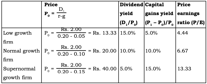
Impact of growth on price, returns, and P/E Ratio
The expected growth rates of companies differ widely. Some companies are expected to remain virtually stagnant or grow slowly; other companies are expected to show normal growth; still others are expected to achieve supernormal growth rate.
Assuming a constant total required return, differing expected growth rates mean differing stock prices, dividend yields, capital gains yields, and price-earnings ratios. To illustrate, consider three cases:
| Growth rate (%) | |
|---|---|
| Low growth firm | 5 |
| Normal growth firm | 10 |
| Supernormal growth firm | 15 |
The expected earnings per share and dividend per share of each of the three firms are Rs. 3.00 and Rs. 2.00 respectively. Investors’ required total return from equity investments is 20 percent.
Given the above information, we may calculate the stock price, dividend yield, capital gains yield, and price-earnings ratio for the three cases as shown in Exhibit 1.
The results in Exhibit 1 suggest the following points:
- As the expected growth in dividend increases, other things being equal, the expected return depends more on the capital gains yield and less on the dividend yield.
- As the expected growth rate in dividend increases, other things being equal, the price- earnings ratio increases.
- High dividend yield and low price-earnings ratio imply limited growth prospects.
- Low dividend yield and high price-earnings ratio imply considerable growth prospects.
Exhibit 1: Price, Dividend Yield, Capital Gains Yield, and Price- Earnings Ratio under Differing Growth Assumptions for 15% Return
Multi-factor share valuation
Quantitative approaches convert a hypothetical relationship between numbers into a unique set of equations. These equations mostly consider company-level data such as market capitalisation, P/E ratio, book-to-price ratio, expectations in earnings, and so on.
Quantitative methods assume that these factors are associated with shares returns, and that certain combinations of these factors can help in assessing the value and, further, predict future values. When several factors are expected to influence share price, a multi-factor model is applied in share valuation.
The choice of the right combination of factors, and how to weigh their relative importance (that is, predicting factor returns) may be achieved through quantitative multivariate statistical tools. Many factors that have been considered individually can be combined to arrive at a best-fit model for valuing equity shares.
Value factors such as price to book, price to sales, and P/E or growth factors such as earnings estimates or earnings per share growth rates, can be used to develop the quantitative model. These quantitative models help to determine what factors best determine valuation during certain market periods. These multifactor share valuation models can also be used to forecast future share values.
Read More Articles