What is Cash Forecasting?
Cash forecasting is an estimation of the flows in and out of the firm’s cash account over a particular period of time, usually a quarter, month, week, or day. The cash forecast is primarily intended to produce a very useful piece of information: an estimation of the firm’s borrowing and lending needs and the uncertainties regarding these needs during various future periods.
Cash forecasting is extremely important to most firms. It enables them to anticipate periods of surplus cash and periods where the financing will be necessary. This anticipation is the reason that cash forecasts are generated. Anticipation enables the firm to plan much more effectively for investment and financing, and via this planning, produce superior returns.
This post highlights design issues relating to forecasting short-term cash flows. We consider both medium-term monthly and quarterly forecasts and daily cash forecasts. We first discuss the benefits and costs of forecasting and then introduce some of the techniques used in cash forecasting systems.
Table of Contents
Cash Forecasting Type
Cash forecasting may be divided into roughly three sub-problems. Depending on the horizon the forecaster wishes to consider. Different techniques and purposes are associated with each horizon.
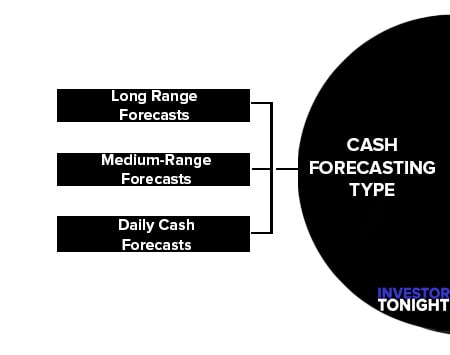
Long Range Forecasts
Cash forecasts of 1 or more years into the future are needed primarily to assess the viability of the firm’s long-range financing and operating policies. Long-range forecasts give planners an idea of how much cash the firm needs to raise through debt or equity issues, internally generated cash or other cash sources.
These forecasts also assist managers in establishing dividend policies, determining capital investments, and planning a mergers and acquisitions (or divestitures) programme. It is typical for a firm to have a 5 or 10-year forecast that is updated annually.
Long-range forecasts are generally based on accounting projections and typically involved the generation of various scenarios for future economic and technological environments. Such forecasts are considered strategic in the sense that possible major changes are examined.
Medium-Range Forecasts
We consider medium-range forecasts to be those that cover cash flows during the next 12 months. A firm may have, for example, a forecast of quarterly cash flows over the next 4 quarters, with monthly detail over the next 3 months. Medium-range cash forecasting usually takes the firm’-S existing technology and long-range financing as given. Hence, this kind of forecast is considered tactical rather than strategic.
Although it can be accounting based, adjustments are made to focus on cash flows rather than earnings. It is sometimes called cash budgeting. The purpose of medium-range forecasting is to determine the firms need for short-term cash from credit lines, commercial paper sales, or credit and payables policies. It also helps firms to determining the makeup of their short-term investment portfolio.
When a firm performs the task called budgeting, it generally designates the most likely (or most desirable) scenario of the medium-range forecasts as the budget. The budget is used to compare actual performance during the course of the year.
Daily Cash Forecasts
Daily cash forecasts attempt to project cash inflows and outflows on a daily basis 1 or more days into the future. This is perhaps the most difficult forecasting to perform accurately. Even though a firm may know precisely its revenues for the month, it may have difficulty determining specific cash inflows for given days of the month.
For some firms, A daily forecast several months into the future is possible. For most, however, a forecast even 2 days into the future is difficult. The purposes of daily forecasting are to assist management in scheduling transfer in cash concentration, funding disbursement accounts, controlling field deposits, and making short-term investing and borrowing decisions.
Objectives of Cash Forecasting
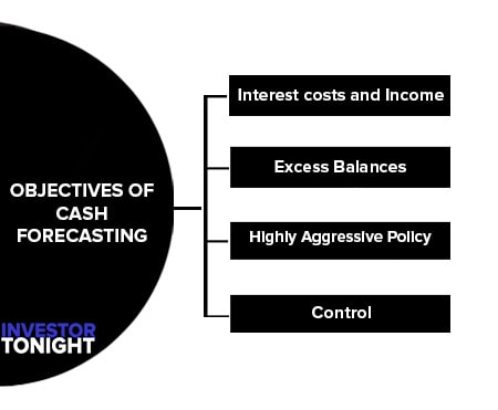
Interest costs and Income
One major purpose of forecasting is to increase the firm’s yield on its investment portfolio or depending on the firm’s financial position, to decrease interest costs on its borrowing. Lack of an accurate forecast may force management either to invest in very short-term securities (thereby often earning the lowest yields) or to borrow unexpectedly at higher than usual interest rates.
Excess Balances
This may be considered a corollary to the first factor. Accurate daily cash forecasts enable management to reduce balances in disbursement and/or deposit accounts and thereby move otherwise non-interest- earning cash into other areas of the firm.
Administrative Costs Benefits
Forecasting may require extensive administrative efforts to collect and digest data. On the other hand, forecasting may provide administrative benefits in the form of better planning and more timely management reports.
Control
Daily cash budgets often provide a standard against which deposit reports from the field can be compared. If actual deposit vary from project deposits, inquiries may be warranted. 5. Forecast System Costs: There costs are associated directly with developing, maintaining, and running the forecasting model and associated data bases. Some forecast systems require extensive computer time and information. Others are simple and inexpensive.
Designing forecasting systems requires that management make trade off among these five cost factors. For example, an extensive, accurate forecasting system may be costly to build and maintain and may require strong administrative effort.
But such a system may enable the firm to achieve better returns on its short-term investments, reduce borrowing costs, and exert better control over cash flows. To determine whether such a system is worth the cost, a detailed study would be conducted to qualify the five factors.
Methods of Financial Forecasting
Financial forecasting is the estimation of the future level of a financial variable, often a cash flow, asset level, or liability level. It is usually assumed that the relationship between the financial variable and other variables is linear. The general linear model can then be used.
Yt = aa + a1 X1 + a2 X2 ………. an Xn ———————(1)
Here, Y is the financial variable (Y) to be forecast in period t. This X’s are the explanatory variables, they are assumed to cause the level of Y in period t. The a term represents a constant unaffected by the X’s. The other a terms are the estimated Coefficients of the explanatory X variables.
There are n terms with X’s in them. This general methodology will be clearer as examples are presented. It is understood that any forecast made in this way is subject to some prediction error because of uncertainty about the exact relationship between the explanatory variables (the X’s) and the outcome variable (the Y; that is, uncertainty about the a coefficients).
There are four common approaches to forecasting financial variables, but they are all special cases of the general linear model.
These four methods of financial forecasting are discussed below:
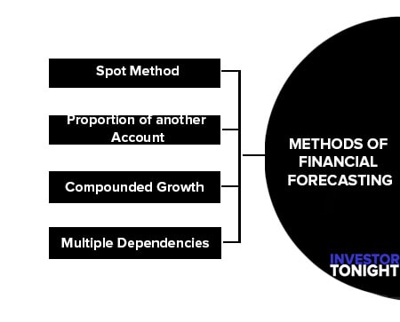
Spot Method
Here it is assumed that the variable to be forecast is independent of all other variables, or alternatively, is predetermined. The variable is forecast by using its expected or predetermined level. All other explanatory variables are presumed to be irrelevant and the formula used is
Y1 = a0 ——————— (2)
where a is the expected or predetermined level of Y. For example, if we are doing a cash forecast and we know that the level of particular types of disbursement (such as rental payments) will be Rs. 12,000 in every month because of the firm’s lease agreement, it would be reasonable to use the spot method to estimate rental payments as Rs. 12,000 per month.
Proportion of another Account
This technique is used to project financial variables that are expected to vary directly with the level of another variable. The formula used is:
Y1 = a1 X1——————— (3)
where X1 is the other variable to which Y is related and a1 is the constant of proportionality between the two. The “percent of sales” method is a variation of this technique, wherein X1 is sales for a particular period and a1 is the percent. The “proportion of another account” method is widely used, when there is a causal link from the explanatory variable to the variable to be forecast.
For example, if sales volume (units sold) increases, it is natural that more units will have to be produced to replenish inventory. It is then reasonable to project certain direct costs of production, such as direct materials, as a percent of sales.
In this circumstance, if costs of direct materials have historically been 50 percent of sales, and sales for a particular period have been forecast as Rs. 1,00,000, the firm would normally project direct material purchases at Rs. 50,000 for that period
Compounded Growth
This method is used when a particular financial variable is expected to grow at a steady growth rate over time. The formula is the same as equation (3), but the explanatory variable X1 is the prior period’s level of Y, and a is one plus the expected growth rate. That is:
Yt = (1+g) Yt-1 ———————(4)
Where g is the period’s growth rate. For example, if it is expected that a firm’s level of selling expenses will grow at 10 percent per year, and this year’s selling expenses are Rs. 10,00,000, we would project next year’s selling expenses as Rs, 1,00,000.
Multiple Dependencies
Here the variable is thought to depend on more than one factor; not just sales or some other variable but a combination of several variables. The general linear model as expressed in equation (1) is used, and the statistical technique of linear regression is often employed with historic data to estimate which explanatory variables are significant in determining Y and to estimate the coefficients of these variables.
A classic example of multiple dependency is inventory level. Finns often keep a “base level” or “safety stock” of inventory to hedge uncertainty and vary the remaining portion of inventory in response to demand. In such a system, there are two appropriate variables associated with inventory level:
Yt = a0 + a1 X1 ———————(5)
There a0 term represents the base inventory level, the Xt the square root of the sales level, and at the proportionality constant. If the firm’s base level of inventory is Rs. 50,000, the proportionality constant is 15 and sales are expected to be Rs. 5,00,000, we could estimate inventory as:
Yt = 50,000 + (15) ((500,000)1/2) = Rs. 60,607
In deciding which of these methods to use to forecast a particular variable, a primary consideration is the term of the forecast: how far into the future are we projecting? To see this, the concepts of the short run and the long run from economics can be employed.
In the short run, most things are predetermined or preplanned; very little can be changed. In the long run, almost everything is variable.
In terms of financial forecasting, this means that in short-term forecasts, many things will result from plans and events that are already in place (contracts, capital budgets, long-range financing plans, and so forth). But in the long run, most things can vary and are dependent on outside influences such as the firm’s long-term growth rate.
Since cash forecasts deal mostly with the near future, many of the items on the cash forecast are estimated by some variation of the spot method. The bases for these spot estimates are usually the firm’s other financial plans.
The remaining estimates are mostly in a “proportion of another account” basis, with this “other account” often being a particular period’s scales; the other two methods are employed less frequently. This is quite unlike longer-term forecasting. Where compounded growth and multiple dependency methodologies play a more important role